Notations

 

I =  number of instruments in portfolio; i = {1,…,I} index of instruments in portfolio;

J =  number of scenarios; j = {1,…,J} index of scenarios;

=  portion of wealth invested in instrument i, i = {1,…,I};

=  vector of decision variables;

= lower bound on portion of wealth invested in instrument i, i = {1,…,I};

= upper bound on wealth invested in instrument i, i = {1,…,I};

= price of instrument i at initial time 0;

= price-vector at initial time 0;

=  price of instrument i for scenario j at time 1;

= rate of return of instrument i for scenario j;

= return of instrument i for scenario j;

= random value having J equally probable scenarios of rates of return, ;

= random value having J equally probable scenarios of  returns,

= random vector of rates of return;

= random return vector;

= vector of rates of return for scenario j;

= return vector  for scenario j;

 

 

 

 

function, where w is a threshold value;

 

 

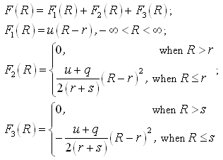
F(R) = an appraisal (= monitoring) function, a linear-quadratic function modeling the decision maker attitude towards risk.

F(R) is defined as follows:

r = the hurdle rate;

s = the sub-hurdle rate, s < r;

u, q =constants, q < - u < 0;

The function F(R) can be represented as follows:

 

 

Optimization Problem 1

 

Maximizing Exponential Utility

 

subject to

 

budget constraint

bounds on positions

 

 

Optimization Problem 2

 

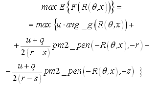
Maximizing Linear-Quadratic Utility

 

 

subject to

 

budget constraint

bounds on positions

 

 

Optimization Problem 3

 

Maximizing Logarithmic Utility

 

 

subject to

 

budget constraint

bounds on positions

 

 

Initial Data

 

Number of instruments in the portfolio, I = 12;

Number of scenarios, J = 199554;

Values of parameters:

q = -20;

u = 1;

r = 10;

s = 3.