Sum of Splines in Optimization
Spline_Sum Operator as input argument for risk functions based on loss scenarios in optimization problems (see Extended Mathematical Definition).
Additional constraint in Optimization problem
Examples of Optimization Problem
Case Studies with Sum of Splines
risk_function(spline_sum(matrix_param, matrix_data)) |
short call; |
risk_function(spline_sum(matrix_param, matrix_data, matrix_knots)) |
call with matrix of knots; |
risk_function_name(spline_sum(matrix_param, matrix_data, matrix_knots)) |
call with matrix of knots and optional name. |
risk_function PSG risk function based on vector of loss scenarios;
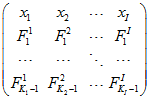
matrix_param is a PSG matrix:

where
header row contains names of factors ![]() . Other rows contain numerical data:
. Other rows contain numerical data:
![]() = degrees of polynomial function for each factor.
= degrees of polynomial function for each factor.
![]() = numbers of polynomial spline pieces for each factor.
= numbers of polynomial spline pieces for each factor.
![]() = smoothing degree for spline for each factor.
= smoothing degree for spline for each factor.
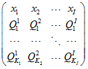
matrix_data is a Matrix of Scenarios:

where
header row contains names of factors ![]() (except scenario_probability, and scenario_benchmark). Other rows contain numerical data. The scenario_probability, and scenario_benchmark columns are optional.
(except scenario_probability, and scenario_benchmark). Other rows contain numerical data. The scenario_probability, and scenario_benchmark columns are optional.
matrix_knots is a PSG matrix:

where
header row contains names of factors. Other rows contain numerical data (set of knots).
Remarks
| • | matrix_knots contain (user specified) values of knots and this matrix is optional. If a set of knots is not specified (for all variables or for some of them) then knots are automatically generated; |
| • | number of knot for every variable should be equal to the number of pieces minus 1 ( |
| • | number of knot values in one column of matrix_knots may differ from the number of knot values in another column ( |
point point with two columns:

where
first row is predefined (see PSG Point);
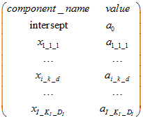
![]() = new variables that define splines coefficients,
= new variables that define splines coefficients, ![]() = number of factor (number of spline),
= number of factor (number of spline), ![]() = number of piece,
= number of piece, ![]() = number of coefficient in polynomial.
= number of coefficient in polynomial.
matrix_data_knots is a PSG matrix:

where
![]() = names of initial (input) variables,
= names of initial (input) variables,
![]() = knots value for i-th variable (spline), and k-th knot,
= knots value for i-th variable (spline), and k-th knot, ![]() ,
, ![]() .
.
Note. If matrix_knots is an input parameter (see Input Argument), then matrix_data_knots = matrix_knots
matrix_data_quants

where
![]() = names of initial (input) variables,
= names of initial (input) variables,
![]() = number of observations between knots
= number of observations between knots ![]() and
and ![]() ,
, ![]() ,
, ![]() .
.
Note. Names of matrix_data_knots and matrix_data_quants consist of two parts: name of matrix matrix_data and suffix _knots or _quants, correspondingly.
Additional Constraints in Optimization Problem
Spline_Sum Operator as an input argument for risk functions in an Optimization problem automatically adds constraints (to the Optimization problem statement). These constraints set smoothness of piecewise polynomial function at knots ![]() ,
, ![]() ,
,![]() .
.
![]() ,
,
where ![]() is the binomial coefficient.
is the binomial coefficient.
Examples of Risk Functions on spline_sum Operator
1. Root Mean Squared Error (st_pen)
Syntax
st_pen(spline_sum(matrix_param, matrix_data, matrix_knots))
Description
![]() = vector with components
= vector with components ![]() ,
,
Standard Penalty PSG function defined on Spline_Sum operator:
 ,
,
where ![]() are described in Extended Mathematical Definition.
are described in Extended Mathematical Definition.
2. Mean Absolute Error (meanabs_pen)
Syntax
meanabs_pen(spline_sum(matrix_param, matrix_data, matrix_knots))
Description
Mean Absolute Penalty PSG function defined on Spline_Sum operator:![]() ,
,
where ![]() are described in Extended Mathematical Definition.
are described in Extended Mathematical Definition.
3. Logarithms Exponents Sum (logexp_sum)
Syntax
logexp_sum(spline_sum(matrix_param, matrix_data, matrix_knots))
Description
Logarithms Exponents Sum PSG function defined on Spline_Sum operator:

![]() ,
,
where ![]() are described in Extended Mathematical Definition.
are described in Extended Mathematical Definition.
Examples of Optimization Problems
Consider two problems of maximization of Logarithms Exponents Sum PSG function defined on:
| 1. | loss operator; |
| 2. | spline_sum operator. |
Problem Statement 1 (loss operator):
maximize
logexp_sum(matrix_data_f1)
Problem Statement 2 (spline_sum operator):
maximize
logexp_sum(spline_sum(matrix_vars_f1, matrix_data_f1))
Solution of two problems in Run-File environment and comprising of outputs:
Table 1. Output files for two problems:
loss operator |
spline_sum operator |
|---|---|
point_problem_1.txt |
point_problem_1.txt |
solution_problem_1.txt |
solution_problem_1.txt |
matrix_data_f1_knots.txt |
|
matrix_data_f1_quant.txt |
Table 2. Solution reports for two problems:
loss operator |
spline_sum operator |
|---|---|
Problem: solution_status = optimal Timing: Data_loading_time = 0.03, Preprocessing_time = 0.00, Solving_time = 0.01 Variables: optimal_point = point_problem_1 Objective: = -0.689382091478 Function: logexp_sum(matrix_data_f1) = -6.893820914784e-001 |
Problem: solution_status = optimal Timing: Data_loading_time = 0.03, Preprocessing_time = 0.01, Solving_time = 0.09 Variables: optimal_point = point_problem_1 Objective: = -0.688993875077 Constraint: constraint_for_smoothing_spline = -6.217248937901e-015 [6.217248937901e-015] Function: logexp_sum(spline_sum(matrix_vars_f1, matrix_data_f1)) = -6.889938750769e-001 |
Note. The constraint_for_smoothing_spline in spline_sum operator is included automatically operator and it is not present in the problem statement (see Additional constraint in Optimization problem).
Table 3. Optimal Points for two problems:
loss operator |
spline_sum operator |
|---|---|
Component_name Value f1 -1.723015759632e-001 f2 -1.617637820650e-002 |
Component_name Value f2_1_1 1.352653430915e+000 f2_1_2 8.427738722586e-001 f2_1_3 1.580275247244e-001 f2_2_0 -6.856379720607e-001 f2_2_1 -2.657989518279e-001 f2_2_2 -4.306815186544e-001 f2_2_3 -1.759723404013e-001 f2_3_0 -6.834447910650e-001 f2_3_1 -2.200513610333e-001 f2_3_2 -1.125983223655e-001 f2_3_3 5.612389385892e-001 f2_4_0 -5.797305765675e-001 f2_4_1 -9.070935285810e-001 f2_4_2 1.404477365784e+000 f2_4_3 -5.553924960276e-001 f2_5_0 -4.196904027755e+000 f2_5_1 7.143498384942e+000 f2_5_2 -4.568144722770e+000 f2_5_3 9.216092365101e-001 intercept 5.064393437277e-001 |
Note. Variable f1 is an intercept and all components of f1 column in matrix_data are equal to 1. In the output of spline_sum operator, f1 variable is automatically renamed to intercept.
Case Studies with Sum of Splines
